Campos vectoriales en diferentes sistemas

De Laplace

(Diferencias entre revisiones)

Revisión de 16:15 25 sep 2008

Contenido

1 Enunciado
2 Solución

1 Enunciado

Exprese los siguientes campos vectoriales en coordenadas cartesianas, cilíndricas y esféricas:

$\mathbf{A} = \mathbf{r}\,$
$\mathbf{B} = -\dfrac{y}{x^2+y^2}\mathbf{u}_{x}+\dfrac{x}{x^2+y^2}\mathbf{u}_{y}$
$\mathbf{C} = 2\rho z\mathbf{u}_{\rho}-(\rho^2-z^2)\mathbf{u}_{z}$
$\mathbf{D}=r\tan\theta\,\mathbf{u}_{\theta}$

2 Solución

2.1 Primer campo

Para expresar el vector de posición en diferentes sistemas coordenados, lo más simple es aplicar que se trata de un gradiente, tal como se ve en otro problema.

Otra posibilidad es el cálculo directo. Por ejemplo, para expresar este vector en coordenadas esféricas, escribimos en primer lugar las componentes cartesianas en función de las coordenadas esféricas

$\mathbf{r}=x\mathbf{u}_{x}+y\mathbf{u}_{y}+z\mathbf{u}_{z}=r\,\mathrm{sen}\,\theta\cos\varphi\mathbf{u}_{x}+r\,\mathrm{sen}\,\theta\mathrm{sen}\varphi\mathbf{u}_{y}+r\cos\theta\mathbf{u}_{z}$

A continuación, multiplicamos por cada uno de los vectores de la base, expresados también en sus componentes cartesianas. La componente radial es

$\mathbf{u}_{r}=\mathrm{sen}\,\theta\cos\varphi\mathbf{u}_{x}+\mathrm{sen}\,\theta\mathrm{sen}\varphi\mathbf{u}_{y}+\cos\theta\mathbf{u}_{z}$

$\mathbf{r}{\cdot}\mathbf{u}_{r}=r(\mathrm{sen}^2\theta\cos^2\varphi+\mathrm{sen}^2\theta\mathrm{sen}^2\varphi+\cos^2\theta)=r$

La componente polar se anula

$\mathbf{u}_{\theta}=\cos\theta\cos\varphi\mathbf{u}_{x}+\cos\theta\mathrm{sen}\varphi\mathbf{u}_{y}-\mathrm{sen}\,\theta\mathbf{u}_{z}$ $\mathbf{r}{\cdot}\mathbf{u}_{\theta}=r(\mathrm{sen}\,\theta\cos\theta\cos^2\varphi+\mathrm{sen}\,\theta\cos\theta\mathrm{sen}^2\varphi-\mathrm{sen}\,\theta\cos\theta)=0$

Lo mismo ocurre con la componente acimutal

$\mathbf{u}_{\varphi}=-\mathrm{sen}\varphi\mathbf{u}_{x}+\cos\varphi\mathbf{u}_{y}$

$\mathbf{r}{\cdot}\mathbf{u}_{\varphi}=r(-\mathrm{sen}\,\theta\cos\varphi\mathrm{sen}\varphi+\mathrm{sen}\,\theta\mathrm{sen}\varphi\cos\varphi)=0$

\] por lo que la expresión final es el conocido

$\mathbf{r}=r\mathbf{u}_{r}$

Una posibilidad adicional de cálculo directo consiste en, tras sustituir las componentes cartesianas por su expresión esféricas, expresar los vectores de la base cartesiana como combinación lineal de los vectores de la base en esféricas. Así, por ejemplo,

$\mathbf{u}_{x}=\mathrm{sen}\,\theta\cos\varphi\mathbf{u}_{r}+\cos\theta\cos\varphi\mathbf{u}_{\theta}-\mathrm{sen}\varphi\mathbf{u}_{\varphi}$

Operando después con los coeficientes de cada vector de la base esférica se llega a la expresión buscada.

2.2 Segundo campo

Para el campo

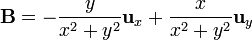
$\mathbf{B}=-\frac{y}{x^2+y^2}\mathbf{u}_{x}+\frac{x}{x^2+y^2}\mathbf{u}_{y}$

podemos sustituir la definición de las coordenadas cilíndricas

$x=\rho\,\cos\varphi$ $y=\rho\,\mathrm{sen}\,\varphi$ $z=z\,$

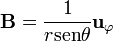
y obtener

$\mathbf{B}=-\frac{\rho\,\mathrm{sen}\,\varphi}{\rho^2}\mathbf{u}_{x}+ \frac{\rho\cos\varphi}{\rho^2}\mathbf{u}_{y} =-\frac{1}{\rho}\left(\mathrm{sen}\,\varphi\mathbf{u}_{x}-\cos\varphi\mathbf{u}_{y}\right)$

el vector que aparece entre paréntesis no es otro que $\mathbf{u}_{\varphi}$ por lo que

$\mathbf{B}=\frac{1}{\rho}\mathbf{u}_{\varphi}$

En esféricas tenemos que, dado que

$\rho=r\,\mathrm{sen}\theta$ $z=r\,\cos\theta$ $\varphi=\varphi$

y que $\mathbf{u}_{\varphi}$ es el mismo en los dos sistemas,

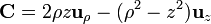
$\mathbf{B}=\frac{1}{r\mathrm{sen}\theta}\mathbf{u}_{\varphi}$

2.3 Tercer campo

Para poner este vector en cartesianas tenemos que

$\mathbf{C}=2z(\rho\mathbf{u}_{\rho})-(\rho^2-z^2)\mathbf{u}_{z}= 2z(x\mathbf{u}_{x}+y\mathbf{u}_{y})-(x^2+y^2-z^2)\mathbf{u}_{z}=2xz\mathbf{u}_{x}+2zy\mathbf{u}_{y}+ (z^2-x^2-y^2)\mathbf{u}_{z}$

y para pasarlo a esféricas resulta

$\mathbf{C}=2r^2\cos\theta\,\mathrm{sen}\,\theta(\mathrm{sen}\,\theta\mathbf{u}_{r}+\cos\theta\mathbf{u}_{\theta})- r^2(\mathrm{sen}^2\theta-\cos^2\theta)(\cos\theta\mathbf{u}_{r}-\mathrm{sen}\,\theta\mathbf{u}_{\theta}) =r^2\cos\theta\mathbf{u}_{r}+r^2\mathrm{sen}\,\theta\mathbf{u}_{\theta}$

@@ Línea 83: / Línea 83: @@
 <center><math>\mathbf{C}=2r^2\cos\theta\,\mathrm{sen}\,\theta(\mathrm{sen}\,\theta\mathbf{u}_{r}+\cos\theta\mathbf{u}_{\theta})-
-r^2(\mathrm{sen}^2\theta-\cos^2\theta)(\cos\theta\mathbf{u}_{r}-\mathrm{sen}\,\theta\mathbf{u}_{\theta})=\]\[
+r^2(\mathrm{sen}^2\theta-\cos^2\theta)(\cos\theta\mathbf{u}_{r}-\mathrm{sen}\,\theta\mathbf{u}_{\theta})
 =r^2\cos\theta\mathbf{u}_{r}+r^2\mathrm{sen}\,\theta\mathbf{u}_{\theta}</math></center>

Campos vectoriales en diferentes sistemas

De Laplace

Revisión de 16:15 25 sep 2008

Contenido

1 Enunciado

2 Solución

2.1 Primer campo

2.2 Segundo campo

2.3 Tercer campo

Herramientas:

Buscar

Vistas

Herramientas

Herramientas personales

Navegación

SEARCH

TOOLBOX

LANGUAGES