


Cálculo de divergencias y rotacionales
De Laplace
(→Campo <math>D</math>) |
(→Campo B) |
||
| (7 ediciones intermedias no se muestran.) | |||
| Línea 10: | Línea 10: | ||
irrotacionales y cuáles solenoidales? | irrotacionales y cuáles solenoidales? | ||
| - | + | ==Campo '''A''' == | |
| - | + | ===Divergencia=== | |
| - | + | ||
| - | + | ||
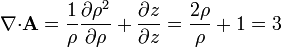
La divergencia, calculada en cartesianas, del vector de posición, es | La divergencia, calculada en cartesianas, del vector de posición, es | ||
| Línea 27: | Línea 25: | ||
<center><math>\nabla{\cdot}\mathbf{A} = \frac{1}{r^2}\frac{\partial (r^3)}{\partial r}= 3</math></center> | <center><math>\nabla{\cdot}\mathbf{A} = \frac{1}{r^2}\frac{\partial (r^3)}{\partial r}= 3</math></center> | ||
| - | + | ===Rotacional=== | |
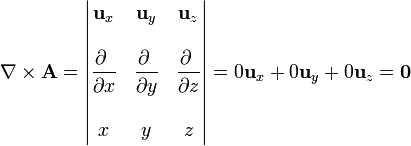
Para el rotacional de este mismo campo, empleando coordenadas cartesianas | Para el rotacional de este mismo campo, empleando coordenadas cartesianas | ||
| Línea 49: | Línea 47: | ||
Naturalmente los resultados son los mismos independientemente del sistema empleado para calcularlos. | Naturalmente los resultados son los mismos independientemente del sistema empleado para calcularlos. | ||
| - | + | ==Campo '''B'''== | |
| - | + | ===Divergencia=== | |
Para el segundo campo, su divergencia, calculada en cartesianas, | Para el segundo campo, su divergencia, calculada en cartesianas, | ||
| Línea 72: | Línea 70: | ||
<center><math>\nabla{\cdot}\mathbf{B} = 0+0+\frac{1}{r\,\mathrm{sen}\,\theta}\frac{\partial \left(r\,\mathrm{sen}\,\theta\right)}{\partial \varphi} = 0</math></center> | <center><math>\nabla{\cdot}\mathbf{B} = 0+0+\frac{1}{r\,\mathrm{sen}\,\theta}\frac{\partial \left(r\,\mathrm{sen}\,\theta\right)}{\partial \varphi} = 0</math></center> | ||
| - | + | ===Rotacional=== | |
Para el rotacional, en cartesianas, | Para el rotacional, en cartesianas, | ||
<center><math>\nabla\times\mathbf{B} = \left|\begin{matrix} | <center><math>\nabla\times\mathbf{B} = \left|\begin{matrix} | ||
| Línea 86: | Línea 84: | ||
y en esféricas | y en esféricas | ||
| - | <center><math>\nabla\times\mathbf{ | + | <center><math>\nabla\times\mathbf{B} = \frac{1}{r^2\mathrm{sen}\,\theta}\left|\begin{matrix}\mathbf{u}_{r} & r\mathbf{u}_{\theta} & r\,\mathrm{sen}\,\theta\mathbf{u}_{\varphi} \\ & & \\ |
\displaystyle \frac{\partial \ }{\partial r} &\displaystyle\frac{\partial \ }{\partial \theta} & \displaystyle\frac{\partial \ }{\partial \varphi} \\ && \\ 0 & 0 & r^2\mathrm{sen}^2\theta\end{matrix}\right|= | \displaystyle \frac{\partial \ }{\partial r} &\displaystyle\frac{\partial \ }{\partial \theta} & \displaystyle\frac{\partial \ }{\partial \varphi} \\ && \\ 0 & 0 & r^2\mathrm{sen}^2\theta\end{matrix}\right|= | ||
2\cos\theta\mathbf{u}_{r}-2\,\mathrm{sen}\,\theta\mathbf{u}_{\theta}</math></center> | 2\cos\theta\mathbf{u}_{r}-2\,\mathrm{sen}\,\theta\mathbf{u}_{\theta}</math></center> | ||
| Línea 92: | Línea 90: | ||
De nuevo el resultado es el mismo aunque, al estar expresado en base diferentes, parece formalmente distinto. | De nuevo el resultado es el mismo aunque, al estar expresado en base diferentes, parece formalmente distinto. | ||
| - | + | ==Campo '''C'''== | |
| - | + | ===Divergencia=== | |
Para el tercer campo, la divergencia en cartesianas | Para el tercer campo, la divergencia en cartesianas | ||
| Línea 116: | Línea 114: | ||
<center><math>\nabla{\cdot}\mathbf{C} = 3(3\cos^2\theta-1)-3(\mathrm{sen}^2\theta-2\cos^2\theta)=0</math></center> | <center><math>\nabla{\cdot}\mathbf{C} = 3(3\cos^2\theta-1)-3(\mathrm{sen}^2\theta-2\cos^2\theta)=0</math></center> | ||
| - | + | ===Rotacional=== | |
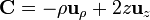
Para el rotacional, en cartesianas | Para el rotacional, en cartesianas | ||
| - | <center><math>\nabla\times\mathbf{ | + | <center><math>\nabla\times\mathbf{C} = \left|\begin{matrix} |
\mathbf{u}_{x} & \mathbf{u}_{y} & \mathbf{u}_{z} \\ & & \\ | \mathbf{u}_{x} & \mathbf{u}_{y} & \mathbf{u}_{z} \\ & & \\ | ||
\displaystyle\frac{\partial \ }{\partial x} & \displaystyle\frac{\partial \ }{\partial y} & \displaystyle\frac{\partial \ }{\partial z} \\ && \\ -x & -y & 2z\end{matrix}\right|= | \displaystyle\frac{\partial \ }{\partial x} & \displaystyle\frac{\partial \ }{\partial y} & \displaystyle\frac{\partial \ }{\partial z} \\ && \\ -x & -y & 2z\end{matrix}\right|= | ||
| Línea 126: | Línea 124: | ||
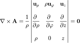
En cilíndricas | En cilíndricas | ||
| - | <center><math>\nabla\times\mathbf{ | + | <center><math>\nabla\times\mathbf{C} = \frac{1}{\rho}\left|\begin{matrix}\mathbf{u}_{\rho} & \rho\mathbf{u}_{\varphi} & \mathbf{u}_{z} \\ & & \\ |
\displaystyle\frac{\partial \ }{\partial \rho} &\displaystyle\frac{\partial \ }{\partial \varphi} & \displaystyle\frac{\partial \ }{\partial z} \\ && \\ -\rho & 0 & 2z\end{matrix}\right|= | \displaystyle\frac{\partial \ }{\partial \rho} &\displaystyle\frac{\partial \ }{\partial \varphi} & \displaystyle\frac{\partial \ }{\partial z} \\ && \\ -\rho & 0 & 2z\end{matrix}\right|= | ||
\mathbf{0}</math></center> | \mathbf{0}</math></center> | ||
| Línea 132: | Línea 130: | ||
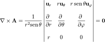
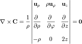
y en esféricas | y en esféricas | ||
| - | <center><math>\nabla\times\mathbf{ | + | <center><math>\nabla\times\mathbf{C} = \frac{1}{r^2\mathrm{sen}\,\theta}\left|\begin{matrix}\mathbf{u}_{r} & r\mathbf{u}_{\theta} & r\,\mathrm{sen}\,\theta\mathbf{u}_{\varphi} \\ & & \\ |
\displaystyle \frac{\partial \ }{\partial r} &\displaystyle\frac{\partial \ }{\partial \theta} & \displaystyle\frac{\partial \ }{\partial \varphi} \\ && \\ r(3\cos^2\theta-1) & -3r^2\mathrm{sen}\,\theta\cos\theta & 0\end{matrix}\right|= | \displaystyle \frac{\partial \ }{\partial r} &\displaystyle\frac{\partial \ }{\partial \theta} & \displaystyle\frac{\partial \ }{\partial \varphi} \\ && \\ r(3\cos^2\theta-1) & -3r^2\mathrm{sen}\,\theta\cos\theta & 0\end{matrix}\right|= | ||
\mathbf{0}</math></center> | \mathbf{0}</math></center> | ||
| - | + | ==Campo '''D'''== | |
| - | + | ||
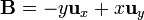
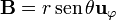
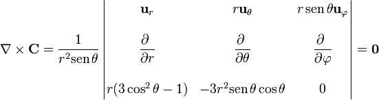
Por último, para el campo | Por último, para el campo | ||
| Línea 145: | Línea 142: | ||
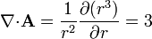
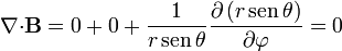
calculamos en primer lugar su divergencia y su rotacional en cilíndricas, ya que en estas coordenadas viene expresado el campo. | calculamos en primer lugar su divergencia y su rotacional en cilíndricas, ya que en estas coordenadas viene expresado el campo. | ||
| - | <center><math>\nabla{\cdot}\mathbf{D} = | + | <center><math>\nabla{\cdot}\mathbf{D} = 3\rho\cos\varphi +\rho\cos\varphi = 4\rho\cos\varphi</math></center> |
| - | <center><math>\nabla\times\mathbf{ | + | <center><math>\nabla\times\mathbf{D} = \frac{1}{\rho}\left|\begin{matrix}\mathbf{u}_{\rho} & \rho\mathbf{u}_{\varphi} & \mathbf{u}_{z} \\ & & \\ |
\displaystyle\frac{\partial \ }{\partial \rho} &\displaystyle\frac{\partial \ }{\partial \varphi} & \displaystyle\frac{\partial \ }{\partial z} \\ && \\ | \displaystyle\frac{\partial \ }{\partial \rho} &\displaystyle\frac{\partial \ }{\partial \varphi} & \displaystyle\frac{\partial \ }{\partial z} \\ && \\ | ||
| - | \rho^2\cos\varphi & \rho^3\mathrm{sen}\varphi & 0\end{matrix}\right| = 4\rho\ | + | \rho^2\cos\varphi & \rho^3\mathrm{sen}\varphi & 0\end{matrix}\right| = 4\rho\mathrm{sen}\varphi\mathbf{u}_{z}</math></center> |
Para calcular estas cantidades en cartesianas, pasamos el campo a este sistema | Para calcular estas cantidades en cartesianas, pasamos el campo a este sistema | ||
| Línea 163: | Línea 160: | ||
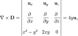
y su rotacional | y su rotacional | ||
| - | + | <center><math>\nabla\times\mathbf{D} = \left|\begin{matrix} | |
\mathbf{u}_{x} & \mathbf{u}_{y} & \mathbf{u}_{z} \\ & & \\ | \mathbf{u}_{x} & \mathbf{u}_{y} & \mathbf{u}_{z} \\ & & \\ | ||
\displaystyle\frac{\partial \ }{\partial x} & \displaystyle\frac{\partial \ }{\partial y} & \displaystyle\frac{\partial \ }{\partial z} \\ && \\ x^2-y^2 & 2xy & 0\end{matrix}\right|= 4y\mathbf{u}_{z}</math></center> | \displaystyle\frac{\partial \ }{\partial x} & \displaystyle\frac{\partial \ }{\partial y} & \displaystyle\frac{\partial \ }{\partial z} \\ && \\ x^2-y^2 & 2xy & 0\end{matrix}\right|= 4y\mathbf{u}_{z}</math></center> | ||
| Línea 175: | Línea 172: | ||
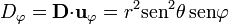
A continuación hallamos las diferentes componentes en esféricas | A continuación hallamos las diferentes componentes en esféricas | ||
| - | <center><math> | + | <center><math>D_r = \mathbf{D}{\cdot}\mathbf{u}_{r}=r^2\mathrm{sen}^3\theta\cos\varphi</math>{{qquad}}<math>D_\theta = \mathbf{D}{\cdot}\mathbf{u}_{\theta}=r^2\mathrm{sen}^2\theta\cos\theta\cos\varphi</math>{{qquad}}<math>D_\varphi = \mathbf{D}{\cdot}\mathbf{u}_{\varphi}=r^2\mathrm{sen}^2\theta\,\mathrm{sen}\varphi</math></center> |
Luego, calculamos los diferentes sumandos que constituyen la divergencia | Luego, calculamos los diferentes sumandos que constituyen la divergencia | ||
| - | <center><math>\frac{1}{r^2}\frac{\partial \ }{\partial r}\left(r^2 | + | <center><math>\frac{1}{r^2}\frac{\partial \ }{\partial r}\left(r^2 D_r\right)=4r\,\mathrm{sen}^3\theta\cos\varphi</math>{{qquad}} |
<math>\frac{1}{r\,\mathrm{sen}\,\theta}\frac{\partial \ }{\partial \theta}\left(\mathrm{sen}\theta | <math>\frac{1}{r\,\mathrm{sen}\,\theta}\frac{\partial \ }{\partial \theta}\left(\mathrm{sen}\theta | ||
| - | + | D_\theta\right)=r\cos\varphi(3\,\mathrm{sen}\theta\cos^2\theta-\mathrm{sen}^3\theta)</math>{{qquad}} | |
| - | <math>\frac{1}{r\,\mathrm{sen}\,\theta}\frac{\partial \ }{\partial \varphi}( | + | <math>\frac{1}{r\,\mathrm{sen}\,\theta}\frac{\partial \ }{\partial \varphi}(D_\varphi)=r\,\mathrm{sen}\,\theta\cos\varphi</math></center> |
y, por último, sumamos | y, por último, sumamos | ||
| - | <center><math>\nabla{\cdot}\mathbf{ | + | <center><math>\nabla{\cdot}\mathbf{D}=4r\,\mathrm{sen}\,\theta\cos\varphi</math></center> |
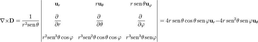
Para el rotacional | Para el rotacional | ||
| - | <center><math>\nabla\times\mathbf{ | + | <center><math>\nabla\times\mathbf{D} = \frac{1}{r^2\mathrm{sen}\,\theta}\left|\begin{matrix}\mathbf{u}_{r} & r\mathbf{u}_{\theta} & r\,\mathrm{sen}\,\theta\mathbf{u}_{\varphi} \\ & & \\ |
\displaystyle \frac{\partial \ }{\partial r} &\displaystyle\frac{\partial \ }{\partial \theta} & \displaystyle\frac{\partial \ }{\partial \varphi} \\ && \\ | \displaystyle \frac{\partial \ }{\partial r} &\displaystyle\frac{\partial \ }{\partial \theta} & \displaystyle\frac{\partial \ }{\partial \varphi} \\ && \\ | ||
r^2\mathrm{sen}^3\theta\cos\varphi & r^3\mathrm{sen}^2\theta\cos\theta\cos\varphi & | r^2\mathrm{sen}^3\theta\cos\varphi & r^3\mathrm{sen}^2\theta\cos\theta\cos\varphi & | ||
| Línea 203: | Línea 200: | ||
puede verse que los tres resultados son coincidentes. | puede verse que los tres resultados son coincidentes. | ||
| - | |||
[[Categoría:Problemas de fundamentos matemáticos]] | [[Categoría:Problemas de fundamentos matemáticos]] | ||
última version al 08:50 13 oct 2010
Contenido |
1 Enunciado
Para los campos vectoriales


calcule su divergencia y su rotacional, empleando en cada caso, coordenadas cartesianas, cilíndricas y esféricas. ¿Cuáles son irrotacionales y cuáles solenoidales?
2 Campo A
2.1 Divergencia
La divergencia, calculada en cartesianas, del vector de posición, es

Para este mismo campo, en cilíndricas, sustituyendo la expresión de  dada en otro problema
y, en esféricas,
2.2 Rotacional
Para el rotacional de este mismo campo, empleando coordenadas cartesianas
en cilíndricas
y en esféricas
Naturalmente los resultados son los mismos independientemente del sistema empleado para calcularlos.
3 Campo B
3.1 Divergencia
Para el segundo campo, su divergencia, calculada en cartesianas,

En cilíndricas este campo se escribe

y la divergencia

En esféricas el campo es
y la divergencia
3.2 Rotacional
Para el rotacional, en cartesianas,

En cilíndricas

y en esféricas

De nuevo el resultado es el mismo aunque, al estar expresado en base diferentes, parece formalmente distinto.
4 Campo C
4.1 Divergencia
Para el tercer campo, la divergencia en cartesianas

En cilíndricas, aplicando los resultados del problema de cálculo de gradientes
y el cálculo de la divergencia da

y en esféricas


4.2 Rotacional
Para el rotacional, en cartesianas

En cilíndricas
y en esféricas
5 Campo D
Por último, para el campo
calculamos en primer lugar su divergencia y su rotacional en cilíndricas, ya que en estas coordenadas viene expresado el campo.


Para calcular estas cantidades en cartesianas, pasamos el campo a este sistema

y calculamos su divergencia

y su rotacional
Para pasar a esféricas, primero expresamos  en sus componentes cartesianas

A continuación hallamos las diferentes componentes en esféricas


Luego, calculamos los diferentes sumandos que constituyen la divergencia


y, por último, sumamos

Para el rotacional
Teniendo en cuenta que


puede verse que los tres resultados son coincidentes.

