No Boletín - Otro tiro parabólico (Ex.Sep/15)

De Laplace

Revisión a fecha de 14:07 6 mar 2016; Enrique (Discusión | contribuciones)

(dif) ← Revisión anterior | Revisión actual (dif) | Revisión siguiente → (dif)

1 Enunciado

Un proyectil se mueve en el plano vertical $OXZ\,$ . Se conoce su aceleración constante (debida a su propio peso), y también su posición y su velocidad en el instante inicial ( $t=0\,$ ):

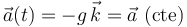
$\vec{a}(t)=-g\,\vec{k}\,\,\,;\,\,\,\,\,\,\,\,\,\,\,\,\vec{r}(0)=h\,\vec{k}\,\,\,; \,\,\,\,\,\,\,\,\,\,\,\,\vec{v}(0)=v_0\,[\,\mathrm{cos}(\theta)\,\vec{\imath}+ \mathrm{sen}(\theta)\,\vec{k}\,]$

donde $g\,$ , $h\,$ y $v_0\,$ tienen valores positivos, y $\theta\,$ está comprendido en el intervalo $0<\theta<\pi/2.\,$

Determine el radio de curvatura de la trayectoria del proyectil en el instante inicial.
Determine la celeridad del proyectil en el instante en el que su trayectoria corta al eje $OX.\,$

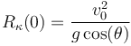
2 Radio de curvatura en el instante inicial

El radio de curvatura de la trayectoria del proyectil en el instante inicial puede calcularse a partir de su velocidad y su aceleración en dicho instante mediante la fórmula:

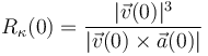
$R_{\kappa}(0)=\frac{|\vec{v}(0)|^3}{|\vec{v}(0)\times\vec{a}(0)|}$

Así que, sustituyendo en dicha fórmula los valores iniciales de velocidad y aceleración:

$\vec{v}(0)=v_0\,[\,\mathrm{cos}(\theta)\,\vec{\imath}+ \mathrm{sen}(\theta)\,\vec{k}\,]\,\,\,;\,\,\,\,\,\,\,\,\,\,\,\,\vec{a}(0)=-g\,\vec{k}$

se obtiene:

$R_{\kappa}(0)=\frac{v_0^2}{g\,\mathrm{cos}(\theta)}$

3 Celeridad del proyectil al cortar el eje OX

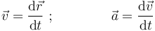
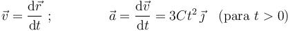
Las definiciones de velocidad instantánea y aceleración instantánea establecen que:

$\vec{v}=\frac{\mathrm{d}\vec{r}}{\mathrm{d}t}\,\, ;\,\,\,\,\,\,\,\,\,\,\,\,\,\,\,\,\,\,\,\,\,\,\,\, \vec{a}=\frac{\mathrm{d}\vec{v}}{\mathrm{d}t}$

En el caso que nos ocupa, conocemos los valores iniciales de la posición $\vec{r}(0)\,$ y de la velocidad $\vec{v}(0)\,$ del proyectil, y además conocemos su aceleración en todo instante, la cual tiene valor constante:

$\vec{a}(t)=-g\,\vec{k}=\vec{a}\,\,\mathrm{(cte)}$

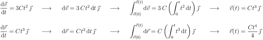
Determinar la velocidad y la posición del proyectil para $t>0\,$ se reduce a integrar la aceleración una y dos veces, respectivamente, entre el instante inicial y un instante genérico:

$\begin{array}{lllll} \mathrm{d}\vec{v}=\vec{a}\,\mathrm{d}t & \,\,\,\,\,\longrightarrow\,\,\,\,\, & \displaystyle\int_{\vec{v}(0)}^{\vec{v}(t)}\!\mathrm{d}\vec{v}=\vec{a}\displaystyle\int_{0}^{t}\mathrm{d}t & \,\,\,\,\,\longrightarrow\,\,\,\,\, & \vec{v}(t)=\vec{v}(0)+\vec{a}\,t \\ \\ \mathrm{d}\vec{r}=[\vec{v}(0)+\vec{a}\,t\,]\,\mathrm{d}t & \,\,\,\,\,\longrightarrow\,\,\,\,\, & \displaystyle\int_{\vec{r}(0)}^{\vec{r}(t)}\!\mathrm{d}\vec{r}=\vec{v}(0)\displaystyle\int_{0}^{t}\mathrm{d}t+\vec{a}\displaystyle\int_{0}^{t}\!t\,\mathrm{d}t & \,\,\,\,\,\longrightarrow\,\,\,\,\, & \vec{r}(t)=\vec{r}(0)+\vec{v}(0)\,t+\displaystyle\frac{1}{2}\,\vec{a}\,t^2\end{array}$

Sustituyendo los valores dados de $\vec{r}(0)\,$ y $\vec{v}(0)\,$ , obtenemos:

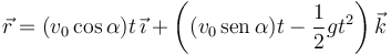
$\vec{v}(t)=v_0\,\mathrm{cos}(\theta)\,\vec{\imath}+\left[v_0\,\mathrm{sen}(\theta)-g\,t\right]\vec{k}\,\,\,;\,\,\,\,\,\,\,\,\,\,\,\,\vec{r}(t)=v_0\,\mathrm{cos}(\theta)\,t\,\vec{\imath}+\left[h+v_0\,\mathrm{sen}(\theta)\,t-\displaystyle\frac{1}{2}\,g\,t^2\right]\vec{k}$

lo que nos da el vector de posición en cada instante

$\vec{r}=(v_0\cos\alpha)t\,\vec{\imath}+\left((v_0\,\mathrm{sen}\,\alpha)t-\frac{1}{2}gt^2\right)\vec{k}$

Derivando el vector de posición respecto al tiempo obtenemos la velocidad intantánea

$\sqrt{v_0^2+2gh}\,$

%%% Conforme a las definiciones de velocidad instantánea y aceleración instantánea, podemos escribir:

$\vec{v}=\frac{\mathrm{d}\vec{r}}{\mathrm{d}t}\,\, ;\,\,\,\,\,\,\,\,\,\,\,\,\,\,\,\,\,\,\,\,\,\,\,\, \vec{a}=\frac{\mathrm{d}\vec{v}}{\mathrm{d}t}=3C t^2\,\vec{\jmath}\,\,\,\,\,\, (\mathrm{para}\,\, t>0)$

Conocemos también las condiciones iniciales de posición y velocidad:

$\vec{r}(0)=\vec{0}\,\mathrm{m}\,\,;\,\,\,\,\,\,\,\,\,\,\,\,\,\,\,\,\,\,\,\,\,\,\,\, \vec{v}(0)=\vec{0}\,\mathrm{m/s}$

Por tanto, determinar la velocidad y la posición de la partícula para $t>0\,$ se reduce a integrar la aceleración una y dos veces, respectivamente, entre el instante inicial y un instante genérico:

$\begin{array}{lllllll}\displaystyle\frac{\mathrm{d}\vec{v}}{\mathrm{d}t}=3C t^2\,\vec{\jmath} & \,\,\,\,\,\longrightarrow\,\,\,\,\, & \mathrm{d}\vec{v}=3\,C t^2\,\mathrm{d}t\,\vec{\jmath} & \,\,\,\,\,\longrightarrow\,\,\,\,\, & \displaystyle\int_{\vec{v}(0)}^{\vec{v}(t)}\!\mathrm{d}\vec{v}=3\,C\left(\displaystyle\int_{0}^{t}\!t^2\,\mathrm{d}t\right)\vec{\jmath} & \,\,\,\,\,\longrightarrow\,\,\,\,\, & \vec{v}(t)=Ct^3\,\vec{\jmath} \\ \\ \displaystyle\frac{\mathrm{d}\vec{r}}{\mathrm{d}t}=Ct^3\,\vec{\jmath} & \,\,\,\,\,\longrightarrow\,\,\,\,\, & \mathrm{d}\vec{r}=Ct^3\,\mathrm{d}t\,\vec{\jmath} & \,\,\,\,\,\longrightarrow\,\,\,\,\, & \displaystyle\int_{\vec{r}(0)}^{\vec{r}(t)}\!\mathrm{d}\vec{r}=C\left(\displaystyle\int_{0}^{t}\!t^3\,\mathrm{d}t\right)\vec{\jmath} & \,\,\,\,\,\longrightarrow\,\,\,\,\, & \vec{r}(t)=\displaystyle\frac{Ct^4}{4}\,\vec{\jmath}\end{array}$

No Boletín - Otro tiro parabólico (Ex.Sep/15)

De Laplace

1 Enunciado

2 Radio de curvatura en el instante inicial

3 Celeridad del proyectil al cortar el eje OX

Herramientas:

Buscar

Vistas

Herramientas

Herramientas personales

Navegación

SEARCH

TOOLBOX

LANGUAGES