


4.1. Estudio de la velocidad de tres puntos
De Laplace
Contenido |
1 Enunciado
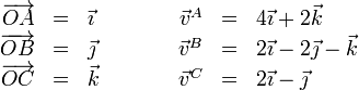
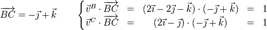
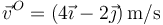
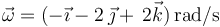
En un hipotético sólido rígido, las posiciones y velocidades de tres puntos son respectivamente:
- Demuestre que estas velocidades son compatibles con la condición de rigidez.
- Halle la velocidad del punto O(0,0,0).
- Calcule la velocidad del punto
 .
.
- ¿Existe algún punto que tenga velocidad nula? ¿Dónde estaría situado?
Todas las cantidades están expresadas en las unidades del SI.
2 Condición de rigidez
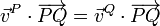
Para que un movimiento sea posible en un sólido rígido debe cumplirse, para todos y cada uno de sus pares de puntos la condición cinemática de rigidez, consistente en la equiproyectividad del campo de velocidades:
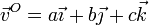
Aplicando esta condición para cada par de partículas resulta:
- Partículas A y B
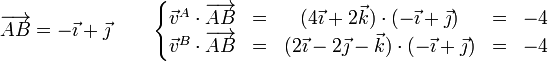
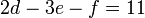
- Partículas A y C
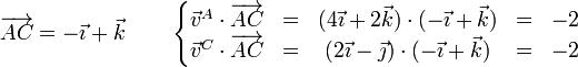
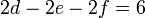
- Partículas B y C
Puesto que los tres pares verifican la condición, estas velocidades son compatibles con un movimiento de un sólido rígido.
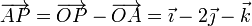
3 Velocidad del origen
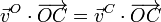
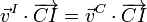
La velocidad de cualquier otro punto se puede obtener aplicando la equiproyectividad con los tres puntos que ya tenemos. Si la velocidad de O es
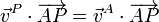
la condición cinemática de rigidez nos da, para el par formado por O y A


Para O y B


Y para O y C

Reuniendo los tres resultados obtenemos la velocidad
4 Velocidad del punto P
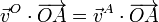
El mismo procedimiento puede emplearse para cualquier otro punto, si bien en general resultará un sistema de ecuaciones lineales. Si la velocidad del punto P es de la forma
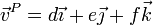
resultan las ecuaciones
Para P y A
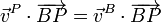
Para P y B

Para P y C

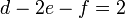
Tenemos entonces el sistema de ecuaciones
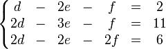
con solución

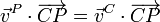
Un procedimiento alternativo para calcular la velocidad de un cuarto punto del sólido rígido, conocidas las velocidades de tres puntos no alineados, consiste en determinar primero el vector velocidad angular  . Las velocidades conocidas están obligadas a satisfacer la ecuación del campo de velocidades. Así, por ejemplo:

Y por otra parte:

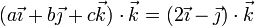
Ya tenemos información suficiente para escribir el vector velocidad angular:
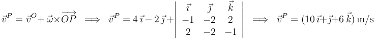
Y ahora, una vez conocido , se puede calcular la velocidad de cualquier punto utilizando de nuevo la ecuación del campo de velocidades:
5 Puntos en reposo instantáneo
5.1 A partir del campo de velocidades
La condición cinemática de rigidez también puede emplearse para hallar posiciones, en lugar de velocidades. En este caso buscamos un punto (o un conjunto de ellos), I, tales que


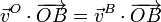
Imponiendo la equiproyectividad con las velocidades de A, B y C tenemos
Para A e I

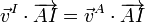

Para B e I

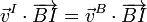

Para C e I


El sistema de ecuaciones para la posición es

Este sistema no siempre tiene solución, ya que si hallamos el rango de los coeficientes, resulta menor que el número de ecuaciones, ya que

por lo que, o no obtenemos solución alguna o resultan infinitas soluciones.
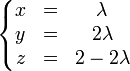
Despejando en la última ecuación


Por tanto obtenemos un conjunto infinito de soluciones, situadas sobre la recta

5.2 Cálculo del EIR
Un procedimiento sistemático para hallar los puntos de velocidad nula es determinar la posición del eje instantáneo de rotación y mínimo deslizamiento (EIRMD) empleando las fórmulas generales.
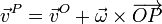
Para ello precisamos calcular en primer lugar la reducción  del campo de velocidades, que nos permite hallar la velocidad de cualquier otro punto como
La velocidad del punto O (que es un punto arbitrario, pero para el que por comodidad tomamos el origen de coordenadas) ya la conocemos. Debemos determinar la velocidad angular del movimiento. Hacemos esto, observando que las velocidades de O, A y B se relacionan como

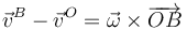
y por tanto la velocidad angular es ortogonal a las dos diferencias de velocidades, por lo que puede escribirse como

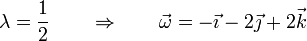
El valor del parámetro λ lo obtenemos a partir de alguno de los pares concretos

de donde
Una vez que conocemos la reducción en el punto O, podemos identificar el movimiento hallando la velocidad de deslizamiento

Por ser nula, se trata de un movimiento de rotación pura. La posición del eje instantáneo de rotación, EIR, se halla mediante la fórmula

Esta ecuación parece diferente de la obtenida anteriormente para los puntos de velocidad nula, pero representa a la misma recta. Si hacemos

se convierte en

que es la misma a la que llegamos antes.

