


4.6. Identificación de posibles movimientos rígidos
De Laplace
1 Enunciado
En un hipotético sólido rígido, consideramos los puntos

y analizamos los casos correspondientes a las siguientes velocidades para los tres puntos:
| Caso | 
| 
| 
|
|---|---|---|---|
| I | 
|
| 
|
| II | 
| 
| 
|
| III | 
|
|
|
| IV | 
| 
| 
|
| V | 
| 
| 
|
| VI |
| 
| 
|
Todas las cantidades están expresadas en las unidades del SI.
Identifique cuáles de las situaciones anteriores son compatibles con la condición de rigidez. Para las que sí lo son, identifique si se trata de un movimiento de traslación pura, rotación pura o helicoidal.
2 Introducción
Para identificar los diferentes estados de movimiento, puesto que lo que se nos da son las velocidades de tres puntos no alineados, es seguir el siguiente esquema:

3 Caso I
Comprobamos primero si se trata de un posible movimiento rígido, chequeando la condición de equiproyectividad para cada par de puntos
- Partículas A y B
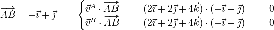
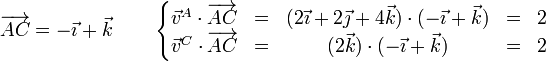
- Partículas A y C
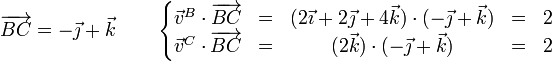
- Partículas B y C
Se verifica en los tres casos, por lo que se trata de un movimiento posible para un sólido rígido.

