Espiral logarítmica

De Laplace

Revisión a fecha de 12:23 26 jun 2010; Antonio (Discusión | contribuciones)

(dif) ← Revisión anterior | Revisión actual (dif) | Revisión siguiente → (dif)

Contenido

1 Enunciado
2 Ley horaria
3 Tiempo en llegar al origen
4 Aceleración
5 Centros de curvatura
- 5.1 Radio de curvatura
- 5.2 Centros de curvatura

1 Enunciado

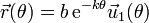
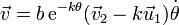
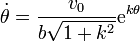
Una partícula recorre la espiral logarítmica de ecuación

$\vec{r} = b (\cos(\theta)\vec{\imath}+\,\mathrm{sen}(\theta)\vec{\jmath})\mathrm{e}^{-k\theta}$

donde $b$ y $k$ son constantes. El movimiento es uniforme a lo largo de la curva, con celeridad constante $v 0$ . En el instante inicial la partícula se encuentra en $θ = 0$

Determine la ley horaria $θ = θ(t)$ .
Calcule el tiempo que tarda en llegar a $\vec{r}=\vec{0}$ . ¿Cuántas vueltas da para ello?
Halle el vector aceleración y sus componentes intrínsecas en cada punto de la trayectoria.
Determine la posición de los centros de curvatura de este movimiento.

2 Ley horaria

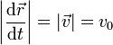
Para hallar la ley horaria $θ = θ(t)$ aplicamos que el movimiento es uniforme y por tanto

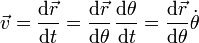
$\left|\frac{\mathrm{d}\vec{r}}{\mathrm{d}t}\right| = |\vec{v}| = v_0$

Sin embargo, lo que se nos da es la trayectoria como función de la coordenada $θ$ y la velocidad no es la derivada de la posición respecto a $θ$ , sino respecto al tiempo. Para relacionar las dos cosas aplicamos la regla de la cadena

$\vec{v}=\frac{\mathrm{d}\vec{r}}{\mathrm{d}t}=\frac{\mathrm{d}\vec{r}}{\mathrm{d}\theta}\,\frac{\mathrm{d}\theta}{\mathrm{d}t}=\frac{\mathrm{d}\vec{r}}{\mathrm{d}\theta}\dot{\theta}$

Aquí $\dot{\theta} =\mathrm{d}\theta/\mathrm{d}t$ es una función que debemos determinar.

Tomando módulos

$v_0= \left|\vec{v}\right|= \left|\frac{\mathrm{d}\vec{r}}{\mathrm{d}\theta}\right|\dot{\theta}$

Derivando en la ecuación de la trayectoria

$\displaystyle\frac{\mathrm{d}\vec{r}}{\mathrm{d}\theta} = b(-\,\mathrm{sen}\,\theta\vec{\imath}+\cos\theta\vec{\jmath})\mathrm{e}^{-k\theta}-bk(\cos\theta\vec{\imath}+\,\mathrm{sen}\,\theta\vec{\jmath})\mathrm{e}^{-k\theta}$

Podemos simplificar esta expresión definiendo dos vectores unitarios

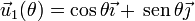
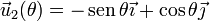
$\vec{u}_1(\theta) = \cos\theta\vec{\imath}+\,\mathrm{sen}\,\theta\vec{\jmath}$ $\vec{u}_2(\theta) = -\,\mathrm{sen}\,\theta\vec{\imath}+\cos\theta\vec{\jmath}$

Estos vectores verifican que son unitarios y ortogonales

$\vec{u}_1\cdot\vec{u}_1=1$ $\vec{u}_2\cdot\vec{u}_2=1$ $\vec{u}_1\cdot\vec{u}_2=0$

y tienen por derivadas

$\frac{\mathrm{d}\vec{u}_1}{\mathrm{d}\theta}=\vec{u}_2$ $\frac{\mathrm{d}\vec{u}_2}{\mathrm{d}\theta}=-\vec{u}_1$

Con ayuda de estos vectores, la posición se expresa

$\vec{r}(\theta)=b\,\mathrm{e}^{-k\theta}\vec{u}_1(\theta)$

y la derivada respecto al ángulo $θ$

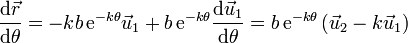
$\frac{\mathrm{d}\vec{r}}{\mathrm{d}\theta}=-k b\,\mathrm{e}^{-k\theta}\vec{u}_1+b\,\mathrm{e}^{-k\theta}\frac{\mathrm{d}\vec{u}_1}{\mathrm{d}\theta}=b\,\mathrm{e}^{-k\theta}\left(\vec{u}_2-k\vec{u}_1\right)$

que es la expresión que ya teníamos, pero más concisa.

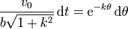
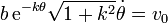
Imponiendo ahora que la celeridad es $v 0$ queda

$v_0 = b\,\mathrm{e}^{-k\theta}\left|\vec{u}_2-k\vec{u}_1\right|\dot{\theta}=b\sqrt{1+k^2}\,\mathrm{e}^{-k\theta}\dot{\theta}$

Para integrar esta ecuación separamos los diferenciales

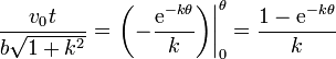
$\frac{v_0}{b\sqrt{1+k^2}}\,\mathrm{d}t = \mathrm{e}^{-k\theta}\,\mathrm{d}\theta$

e integramos, teniendo en cuenta que para $t = 0$ , $θ = 0$

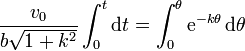
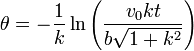
$\frac{v_0}{b\sqrt{1+k^2}}\int_0^t\mathrm{d}t = \int_0^\theta \mathrm{e}^{-k\theta}\,\mathrm{d}\theta$

lo que nos da

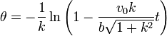
$\frac{v_0 t}{b\sqrt{1+k^2}} = \left.\left(-\frac{\mathrm{e}^{-k\theta}}{k}\right)\right|_0^\theta = \frac{1-\mathrm{e}^{-k\theta}}{k}$

Despejando de aquí

$\theta = -\frac{1}{k}\ln\left(1-\frac{v_0k}{b\sqrt{1+k^2}}t\right)$

3 Tiempo en llegar al origen

El tiempo que tarda la partícula en llegar al origen lo obtenemos exigiendo que $\vec{r}=\vec{0}$ . La posición para cada valor de $θ$ es igual a

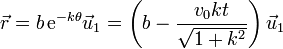
$\vec{r}=b\,\mathrm{e}^{-k\theta}\vec{u}_1 = \left(b-\frac{v_0 k t}{\sqrt{1+k^2}}\right)\vec{u}_1$

Este vector se anulará en

$t = \frac{b\sqrt{1+k^2}}{v_0k}$

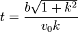
Este es el tiempo en llegar al centro.

Nótese que este valor de $t$ corresponde a un valor de $\theta\to\infty$ . Puesto que $θ$ representa el ángulo que el vector de posición forma con el eje X y que una circunferencia completa significa aumentar $θ$ en $2π$ , vemos que la partícula da infinitas vueltas antes de llegar al origen, aunque para ello requiere un tiempo finito. Igualmente, aunque de infinitas vueltas, la distancia recorrida por la partícula es finita e igual a

$\Delta s = v_0 t = \frac{b\sqrt{1+k^2}}{k}$

Esto es posible porque las suscesivas vueltas son cada vez más pequeñas.

4 Aceleración

4.1 Forma vectorial

Para el cálculo de la aceleración tenemos un problema similar al de la velocidad. La cuestión es que la aceleracion no es la derivada de la velocidad respecto a $θ$ , sino respecto al tiempo, con lo que hay que tener mucho cuidado con qué seriva y respecto a qué.

Partimos de las expresiones que ya conocemos para la velocidad

$\vec{v}=b\,\mathrm{e}^{-k\theta}(\vec{v}_2-k\vec{u}_1)\dot{\theta}$

Conocemos también la ley horaria

$b\,\mathrm{e}^{-k\theta}\sqrt{1+k^2}\dot{\theta}=v_0$ $\Rightarrow$ $\theta=-\frac{1}{k}\ln\left(\frac{v_0kt}{b\sqrt{1+k^2}}\right)$

Una posibilidad sería entonces sustituir $θ(t)$ en la expresión de la velocidad y derivar lo que salga respecto al tiempo. Sin embargo debido a que en esta fórmula aparecen seos y cosenos de logaritmos, la posibilidad de equivocarse al derivar es muy alta.

La solución consiste en aplicar de nuevo la regla de la cadena. Vamos a considerar la velocidad como función del ángulo $θ$ y calcular la aceleración como

$\vec{a}=\frac{\mathrm{d}\vec{v}}{\mathrm{d}t}=\frac{\mathrm{d}\vec{v}}{\mathrm{d}\theta}\,\frac{\mathrm{d}\theta}{\mathrm{d}t}=\frac{\mathrm{d}\vec{v}}{\mathrm{d}\theta}\,\dot{\theta}$

Para ello necesitamos, en primer lugar la velocidad como función de $θ$ , que es algo que aun no tenemos. En la expresión de arriba aparece la velocidad como función de $θ$ y de $\dot{\theta}$ , que no es lo mismo. Debe aparecer solo $θ$ , no las dos cosas.

Despejamos $\dot{\theta}$ como función de $θ$

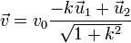
$\dot{\theta}=\frac{v_0}{b\sqrt{1+k^2}}\mathrm{e}^{k\theta}$

y sustituimos en la expresión de la velocidad

$\vec{v}=v_0\frac{\vec{u}_2-k\vec{u}_1}{\sqrt{1+k^2}}$

Esta ya sí solo depende del ángulo $θ$ . Podría parecer que no lo hace, puesto que no aparece en la expresión, pero si está, escondido dentro de los vectores $\vec{u}_1$ y $\vec{u}_2$ , que no son vectores constantes, sino dependientes de la posición (y, por tanto, del tiempo).

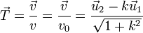
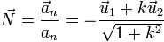
Esta expresión nos dice también que el unitario tangente a la trayectoria es

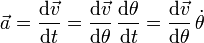
$\vec{T}=\frac{\vec{v}}{v}=\frac{\vec{v}}{v_0}=\frac{\vec{u}_2-k\vec{u}_1}{\sqrt{1+k^2}}$

Aplicando ahora la regla de la cadena para hallar la aceleración tenemos

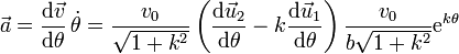
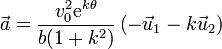
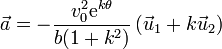
$\vec{a}=\frac{\mathrm{d}\vec{v}}{\mathrm{d}\theta}\,\dot{\theta}=\frac{v_0}{\sqrt{1+k^2}}\left(\frac{\mathrm{d}\vec{u}_2}{\mathrm{d}\theta}-k\frac{\mathrm{d}\vec{u}_1}{\mathrm{d}\theta}\right)\frac{v_0}{b\sqrt{1+k^2}}\mathrm{e}^{k\theta}$

Sustituyendo aquí las derivadas de los vectores unitarios llegamos a

$\vec{a}=\frac{v_0^2\mathrm{e}^{k\theta}}{b(1+k^2)}\left(-\vec{u}_1-k\vec{u}_2\right)$

4.2 Aceleración tangencial

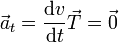
La aceleración tangencial es nula, pues el movimiento es uniforme y su celeridad es constante

$|\vec{v}|=v_0$ $\Rightarrow$ $\frac{\mathrm{d}v}{\mathrm{d}t}=0$ $\Rightarrow$ $\vec{a}_t=\frac{\mathrm{d}v}{\mathrm{d}t}\vec{T}=\vec{0}$

Podemos demostrarlo también a partir de las expresiones vectoriales de la velocidad y la aceleración

$\vec{v}=v_0\frac{-k\vec{u}_1+\vec{u}_2}{\sqrt{1+k^2}}$ $\vec{a}=-\frac{v_0^2\mathrm{e}^{k\theta}}{b(1+k^2)}\left(\vec{u}_1+k\vec{u}_2\right)$

Multiplicando la una por la otra

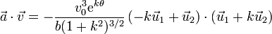
$\vec{a}\cdot\vec{v}=-\frac{v_0^3\mathrm{e}^{k\theta}}{b(1+k^2)^{3/2}}\left(-k\vec{u}_1+\vec{u}_2\right)\cdot\left(\vec{u}_1+k\vec{u}_2\right)$

pero, teniendo en cuenta que $\vec{u}_1$ y $\vec{u}_2$ forman una base ortonormal

$\left(-k\vec{u}_1+\vec{u}_2\right)\cdot\left(\vec{u}_1+k\vec{u}_2\right)=-k+k = 0$

y si la aceleración es perpendicular a la velocidad, la aceleración tangencial, por definición, es nula.

4.3 Aceleración normal

Si la aceleración tangencial es nula, la aceleración normal es toda la aceleración

$\vec{a}_n=\vec{a}=-\frac{v_0^2\mathrm{e}^{k\theta}}{b(1+k^2)}\left(\vec{u}_1+k\vec{u}_2\right)$

Esto nos permite calcular el vector normal a la trayectoria como

$|\vec{a}_n| = \frac{v_0^2\mathrm{e}^{k\theta}}{b(1+k^2)}\sqrt{1+k^2}$ $\Rightarrow$ $\vec{N}=\frac{\vec{a}_n}{a_n} = -\frac{\vec{u}_1+k\vec{u}_2}{\sqrt{1+k^2}}$

5 Centros de curvatura

5.1 Radio de curvatura

Una vez que tenemos la aceleración normal y la celeridad, hallamos el radio de curvatura en cada punto de la trayectoria

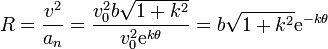
$R = \frac{v^2}{a_n}=\frac{v_0^2 b\sqrt{1+k^2}}{v_0^2\mathrm{e}^{k\theta}} = b\sqrt{1+k^2}\mathrm{e}^{-k\theta}$

Vemos que a medida que disminuye $θ$ , el radio de la curvatura se reduce, lo que corresponde a que la curva es cada vez más cerrada.

5.2 Centros de curvatura

Una vez que tenemos el radio de curvatura y el vector normal, podemos localizar los centros de curvatura

$\vec{r}_c = \vec{r}+R\vec{N}=b\vec{u}_1\mathrm{e}^{-k\theta}+ b\sqrt{1+k^2}\mathrm{e}^{-k\theta}\left(-\frac{\vec{u}_1+k\vec{u}_2}{\sqrt{1+k^2}}\right)=-vk\mathrm{e}^{-k\theta}\vec{u}_2$

Esto quiere decir que el conjunto de los sucesivos centros de curvatura (lo que se denomina técnicamente la evolvente -que no envolvente, que esa es otra-) forma otra espiral logarítmica.

Espiral logarítmica

De Laplace

Contenido

1 Enunciado

2 Ley horaria

3 Tiempo en llegar al origen

4 Aceleración

4.1 Forma vectorial

4.2 Aceleración tangencial

4.3 Aceleración normal

5 Centros de curvatura

5.1 Radio de curvatura

5.2 Centros de curvatura

Herramientas:

Buscar

Vistas

Herramientas

Herramientas personales

Navegación

SEARCH

TOOLBOX

LANGUAGES