Espiral logarítmica

De Laplace

Revisión a fecha de 08:25 25 jun 2010; Antonio (Discusión | contribuciones)

(dif) ← Revisión anterior | Revisión actual (dif) | Revisión siguiente → (dif)

Contenido

1 Enunciado
2 Ley horaria
3 Tiempo en llegar al origen
4 Aceleración
5 Centros de curvatura

1 Enunciado

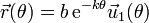
Una partícula recorre la espiral logarítmica de ecuación

$\vec{r} = b (\cos(\theta)\vec{\imath}+\,\mathrm{sen}(\theta)\vec{\jmath})\mathrm{e}^{-k\theta}$

donde $b$ y $k$ son constantes. El movimiento es uniforme a lo largo de la curva, con celeridad constante $v 0$ . En el instante inicial la partícula se encuentra en $θ = 0$

Determine la ley horaria $θ = θ(t)$ .
Calcule el tiempo que tarda en llegar a $\vec{r}=\vec{0}$ . ¿Cuántas vueltas da para ello?
Halle el vector aceleración y sus componentes intrínsecas en cada punto de la trayectoria.
Determine la posición de los centros de curvatura de este movimiento.

2 Ley horaria

Para hallar la ley horaria $θ = θ(t)$ aplicamos que el movimiento es uniforme y por tanto

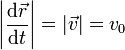
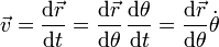
$\left|\frac{\mathrm{d}\vec{r}}{\mathrm{d}t}\right| = |\vec{v}| = v_0$

Sin embargo, lo que se nos da es la trayectoria como función de la coordenada $θ$ y la velocidad no es la derivada de la posición respecto a $θ$ , sino respecto al tiempo. Para relacionar las dos cosas aplicamos la regla de la cadena

$\vec{v}=\frac{\mathrm{d}\vec{r}}{\mathrm{d}t}=\frac{\mathrm{d}\vec{r}}{\mathrm{d}\theta}\,\frac{\mathrm{d}\theta}{\mathrm{d}t}=\frac{\mathrm{d}\vec{r}}{\mathrm{d}\theta}\dot{\theta}$

Aquí $\dot{\theta} =\mathrm{d}\theta/\mathrm{d}t$ es una función que debemos determinar.

Tomando módulos

$v_0= \left|\vec{v}\right|= \left|\frac{\mathrm{d}\vec{r}}{\mathrm{d}\theta}\right|\dot{\theta}$

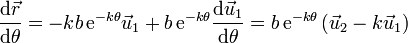
Derivando en la ecuación de la trayectoria

$\displaystyle\frac{\mathrm{d}\vec{r}}{\mathrm{d}\theta} = b(-\,\mathrm{sen}\,\theta\vec{\imath}+\cos\theta\vec{\jmath})\mathrm{e}^{-k\theta}-bk(\cos\theta\vec{\imath}+\,\mathrm{sen}\,\theta\vec{\jmath})\mathrm{e}^{-k\theta}$

Podemos simplificar esta expresión definiendo dos vectores unitarios

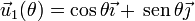
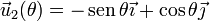
$\vec{u}_1(\theta) = \cos\theta\vec{\imath}+\,\mathrm{sen}\,\theta\vec{\jmath}$ $\vec{u}_2(\theta) = -\,\mathrm{sen}\,\theta\vec{\imath}+\cos\theta\vec{\jmath}$

Estos vectores verifican que son unitarios y ortogonales

$\vec{u}_1\cdot\vec{u}_1=1$ $\vec{u}_2\cdot\vec{u}_2=1$ $\vec{u}_1\cdot\vec{u}_2=0$

y tienen por derivadas

$\frac{\mathrm{d}\vec{u}_1}{\mathrm{d}\theta}=\vec{u}_2$ $\frac{\mathrm{d}\vec{u}_2}{\mathrm{d}\theta}=-\vec{u}_1$

Con ayuda de estos vectores, la posición se expresa

$\vec{r}(\theta)=b\,\mathrm{e}^{-k\theta}\vec{u}_1(\theta)$

y la derivada respecto al ángulo $θ$

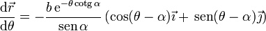
$\frac{\mathrm{d}\vec{r}}{\mathrm{d}\theta}=-k b\,\mathrm{e}^{-k\theta}\vec{u}_1+b\,\mathrm{e}^{-k\theta}\frac{\mathrm{d}\vec{u}_1}{\mathrm{d}\theta}=b\,\mathrm{e}^{-k\theta}\left(\vec{u}_2-k\vec{u}_1\right)$

Aplicando que

$\,\mathrm{sen}\,\theta+\,\mathrm{cotg\alpha}\,\cos\theta = \frac{\,\mathrm{sen}\,\theta\,\mathrm{sen}\,\alpha+\cos\theta\cos\alpha}{\mathrm{sen}\,\alpha}=\frac{\cos(\theta-\alpha)}{\mathrm{sen}\,\alpha}$

y que

$\cos\theta-\,\mathrm{cotg}\,\alpha\,\mathrm{sen}\,\theta = -\frac{\mathrm{sen}\,\theta\cos\alpha-\,\mathrm{sen}\,\alpha\cos\theta}{\mathrm{sen}\,\alpha}=-\frac{\mathrm{sen}(\theta-\alpha)}{\mathrm{sen}\,\alpha}$

obtenemos finalmente

$\frac{\mathrm{d}\vec{r}}{\mathrm{d}\theta} = -\frac{b\,\mathrm{e}^{-\theta\,\mathrm{cotg}\,\alpha}}{\mathrm{sen}\,\alpha}\left(\cos(\theta-\alpha)\vec{\imath}+\,\mathrm{sen}(\theta-\alpha)\vec{\jmath}\right)$

El módulo de esta cantidad es

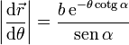
$\left|\frac{\mathrm{d}\vec{r}}{\mathrm{d}\theta}\right| = \frac{b\,\mathrm{e}^{-\theta\,\mathrm{cotg}\,\alpha}}{\mathrm{sen}\,\alpha}$

por lo que llegamos a la condición

$v_0 = \frac{b\,\mathrm{e}^{-\theta\,\mathrm{cotg}\,\alpha}}{\mathrm{sen}\,\alpha}\,\frac{\mathrm{d}\theta}{\mathrm{d}t}$

Para integrar esta ecuación separamos los diferenciales

$v_0\,\mathrm{d}t = \frac{b}{\mathrm{sen}\,\alpha}\mathrm{e}^{-\theta\,\mathrm{cotg}\,\alpha}\,\mathrm{d}\theta$

e integramos, teniendo en cuenta que para $t = 0$ , $θ = 0$

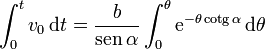
$\int_0^t v_0\,\mathrm{d}t = \frac{b}{\mathrm{sen}\,\alpha}\int_0^\theta \mathrm{e}^{-\theta\,\mathrm{cotg}\,\alpha}\,\mathrm{d}\theta$

lo que nos da

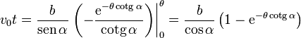
$v_0 t = \frac{b}{\mathrm{sen}\,\alpha}\left.\left(-\frac{\mathrm{e}^{-\theta\,\mathrm{cotg}\,\alpha}}{\mathrm{cotg}\,\alpha}\right)\right|_0^\theta = \frac{b}{\cos\alpha}\left(1-\mathrm{e}^{-\theta\,\mathrm{cotg}\,\alpha}\right)$

Despejando de aquí

$\mathrm{e}^{-\theta\,\mathrm{cotg}\,\alpha}=1-\frac{v_0\cos\alpha}{b}t$ $\Rightarrow$ $\theta = -\mathrm{tg}\,\alpha\ln\left(1-\frac{v_0\cos\alpha}{b}t\right)$

3 Tiempo en llegar al origen

4 Aceleración

5 Centros de curvatura

Espiral logarítmica

De Laplace

Contenido

1 Enunciado

2 Ley horaria

3 Tiempo en llegar al origen

4 Aceleración

5 Centros de curvatura

Herramientas:

Buscar

Vistas

Herramientas

Herramientas personales

Navegación

SEARCH

TOOLBOX

LANGUAGES