Construcción de una base
De Laplace
(→Segundo vector) |
|||
| Línea 13: | Línea 13: | ||
Obtenemos el primer vector normalizando el vector <math>\vec{v}</math>, esto es, hallando el unitario en su dirección y sentido, lo que se consigue dividiendo este vector por su módulo | Obtenemos el primer vector normalizando el vector <math>\vec{v}</math>, esto es, hallando el unitario en su dirección y sentido, lo que se consigue dividiendo este vector por su módulo | ||
| - | <center><math>\vec{T}=\frac{\vec{v}}{v}</math></center> | + | <center><math>\vec{T}=\frac{\vec{v}}{|\vec{v}|}</math></center> |
Hallamos el módulo de <math>\vec{v}</math> | Hallamos el módulo de <math>\vec{v}</math> | ||
| - | <center><math>v = \sqrt{\vec{v}\cdot\vec{v}}=\sqrt{1^2+2^2+2^2}=3</math></center> | + | <center><math> \vec{v}| = \sqrt{\vec{v}\cdot\vec{v}}=\sqrt{1^2+2^2+2^2}=3</math></center> |
por lo que | por lo que | ||
| Línea 40: | Línea 40: | ||
La proyección normal la calculamos con ayuda del [[Vectores_en_física_(GIE)#Doble_producto_vectorial|doble producto vectorial]] | La proyección normal la calculamos con ayuda del [[Vectores_en_física_(GIE)#Doble_producto_vectorial|doble producto vectorial]] | ||
| - | <center><math>\vec{a}_n = \frac{(\vec{v}\times\vec{a})\times\vec{v}}{v^2}</math></center> | + | <center><math>\vec{a}_n = \frac{(\vec{v}\times\vec{a})\times\vec{v}}{|\vec{v}|^2}</math></center> |
Calculamos el primer producto vectorial | Calculamos el primer producto vectorial | ||
| Línea 60: | Línea 60: | ||
Normalizando esta cantidad obtenemos el segundo vector de la base | Normalizando esta cantidad obtenemos el segundo vector de la base | ||
| - | <center><math>\vec{N} = \frac{\vec{a}_n}{ | + | <center><math>\vec{N} = \frac{\vec{a}_n}{|\vec{a}_n|}=\frac{2}{3}\vec{\imath}+\frac{1}{3}\vec{\jmath}-\frac{2}{3}\vec{k}</math></center> |
==Tercer vector== | ==Tercer vector== | ||
El tercer vector lo obtenemos como el producto vectorial de los dos primeros | El tercer vector lo obtenemos como el producto vectorial de los dos primeros | ||
| - | <center><math>\vec{ | + | <center><math>\vec{B}=\vec{T}\times\vec{N}=\left|\begin{matrix}\vec{\imath} & \vec{\jmath} & \vec{k} \\ 1/3 & 2/3 & 2/3 \\ 2/3 & 1/3 & -2/3\end{matrix}\right|=\frac{1}{9}\left|\begin{matrix}\vec{\imath} & \vec{\jmath} & \vec{k} \\ 1 & 2 & 2 \\ 2 & 1 & -2\end{matrix}\right| = -\frac{2}{3}\vec{\imath}+\frac{2}{3}\vec{\jmath}-\frac{1}{3}\vec{k}</math></center> |
Por tanto, la base ortonormal dextrógira está formada por los vectores | Por tanto, la base ortonormal dextrógira está formada por los vectores | ||
| Línea 71: | Línea 71: | ||
<center><math> | <center><math> | ||
\begin{array}{lcr} | \begin{array}{lcr} | ||
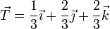
| - | \vec{ | + | \vec{T} & = & \displaystyle\frac{1}{3}\vec{\imath}+\displaystyle\frac{2}{3}\vec{\jmath}+\displaystyle\frac{2}{3}\vec{k}\\&& \\ |
| - | \vec{ | + | \vec{N} & = & \displaystyle\frac{2}{3}\vec{\imath}+\displaystyle\frac{1}{3}\vec{\jmath}-\displaystyle\frac{2}{3}\vec{k}\\&& \\ |
| - | \vec{ | + | \vec{B} & = & -\displaystyle\frac{2}{3}\vec{\imath}+\displaystyle\frac{2}{3}\vec{\jmath}-\displaystyle\frac{1}{3}\vec{k} |
\end{array}</math></center> | \end{array}</math></center> | ||
| Línea 81: | Línea 81: | ||
El tercer vector de la base es ortogonal a los dos primeros. También es ortogonal a cualquier combinación lineal de los dos primeros, en particular a los dos vectores del enunciado <math>\vec{v}</math> y <math>\vec{a}</math>. Por ello, podemos calcular el tercer vector como | El tercer vector de la base es ortogonal a los dos primeros. También es ortogonal a cualquier combinación lineal de los dos primeros, en particular a los dos vectores del enunciado <math>\vec{v}</math> y <math>\vec{a}</math>. Por ello, podemos calcular el tercer vector como | ||
| - | <center><math>\vec{ | + | <center><math>\vec{B} = \frac{\vec{v}\times\vec{a}}{|\vec{v}\times\vec{a}|}</math></center> |
El producto vectorial vale | El producto vectorial vale | ||
| Línea 93: | Línea 93: | ||
resultando el unitario | resultando el unitario | ||
| - | <center><math>\vec{ | + | <center><math>\vec{B} = -\frac{2}{3}\vec{\imath}+\frac{2}{3}\vec{\jmath}-\frac{1}{3}\vec{k}</math></center> |
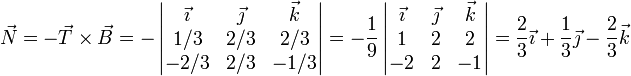
El segundo vector lo obtenemos del producto vectorial del primero y el tercero, teniendo en cuenta el cambio de signo debido a la inversión del orden | El segundo vector lo obtenemos del producto vectorial del primero y el tercero, teniendo en cuenta el cambio de signo debido a la inversión del orden | ||
| - | <center><math>\vec{ | + | <center><math>\vec{N} = -\vec{T}\times\vec{B} = -\left|\begin{matrix}\vec{\imath} & \vec{\jmath} & \vec{k} \\ 1/3 & 2/3 & 2/3 \\ -2/3 & 2/3 & -1/3\end{matrix}\right|=-\frac{1}{9}\left|\begin{matrix}\vec{\imath} & \vec{\jmath} & \vec{k} \\ 1 & 2 & 2 \\ -2 & 2 & -1\end{matrix}\right| = \frac{2}{3}\vec{\imath}+\frac{1}{3}\vec{\jmath}-\frac{2}{3}\vec{k}</math></center> |
[[Categoría:Problemas de herramientas matemáticas (GIE)]] | [[Categoría:Problemas de herramientas matemáticas (GIE)]] | ||
Revisión de 14:51 4 oct 2011
Contenido |
1 Enunciado
Dados los vectores

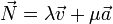
Construya una base ortonormal dextrógira  , tal que
- El primer vector,
 , vaya en la dirección y sentido de
- El segundo,
 , esté contenido en el plano definido por y
  y apunte hacia el mismo semiplano (respecto de ) que el vector .
- El tercero,
 , sea perpendicular a los dos anteriores, y orientado según la regla de la mano derecha.
2 Primer vector
Obtenemos el primer vector normalizando el vector , esto es, hallando el unitario en su dirección y sentido, lo que se consigue dividiendo este vector por su módulo

Hallamos el módulo de

por lo que
3 Segundo vector
El segundo vector debe estar en el plano definido por y , por lo que debe ser una combinación lineal de ambos
además debe ser ortogonal a (y por tanto, a )
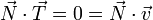
y debe ser unitario

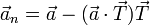
El procedimiento sistemático consiste en hallar la componente de perpendicular a y posteriormente normalizar el resultado.
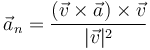
La proyección normal la calculamos con ayuda del doble producto vectorial
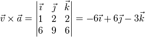
Calculamos el primer producto vectorial
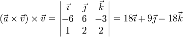
Hallamos el segundo
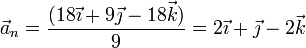
Dividiendo por el módulo de al cuadrado obtenemos la componente normal
Alternativamente, podemos hallar esta proyección ortogonal restando al vector completo la parte paralela
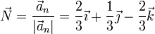
Normalizando esta cantidad obtenemos el segundo vector de la base
4 Tercer vector
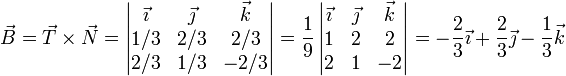
El tercer vector lo obtenemos como el producto vectorial de los dos primeros
Por tanto, la base ortonormal dextrógira está formada por los vectores
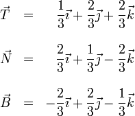
5 Forma alternativa
Podemos acortar un poco el proceso invirtiendo el orden de cálculo.
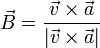
El tercer vector de la base es ortogonal a los dos primeros. También es ortogonal a cualquier combinación lineal de los dos primeros, en particular a los dos vectores del enunciado y . Por ello, podemos calcular el tercer vector como
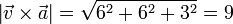
El producto vectorial vale
con módulo
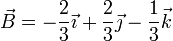
resultando el unitario
El segundo vector lo obtenemos del producto vectorial del primero y el tercero, teniendo en cuenta el cambio de signo debido a la inversión del orden