


4.6. Identificación de posibles movimientos rígidos
De Laplace
(→Caso IV) |
(→Caso I) |
||
| Línea 77: | Línea 77: | ||
A continuación, comprobamos si las tres velocidades son iguales. No lo son. Por tanto, no puede tratarse de una traslación o un estado de reposo. | A continuación, comprobamos si las tres velocidades son iguales. No lo son. Por tanto, no puede tratarse de una traslación o un estado de reposo. | ||
| - | Comprobamos ahora si hay dos velocidades iguales. Las hay. Esto quiere decir que el EIRMD es paralelo a la recta que pasa por los dos puntos con la misma velocidad. Para ver si se trata de una rotación, examinamos si cualquiera de las velocidades | + | Comprobamos ahora si hay dos velocidades iguales. Las hay. Esto quiere decir que el EIRMD es paralelo a la recta que pasa por los dos puntos con la misma velocidad. Para ver si se trata de una rotación, examinamos si cualquiera de las velocidades es perpendicular a esta dirección. No necesitamos volver a calcular nada, ya que lo hicimos previamente: |
<center><math>\vec{v}^A\cdot\overrightarrow{AB}=0</math></center> | <center><math>\vec{v}^A\cdot\overrightarrow{AB}=0</math></center> | ||
Revisión de 21:22 13 nov 2010
Contenido |
1 Enunciado
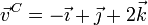
En un hipotético sólido rígido, consideramos los puntos

y analizamos los casos correspondientes a las siguientes velocidades para los tres puntos:
| Caso | 
| 
| 
|
|---|---|---|---|
| I | 
|
| 
|
| II | 
| 
| 
|
| III | 
|
|
|
| IV | 
| 
| 
|
| V | 
| 
| 
|
| VI |
| 
| 
|
Todas las cantidades están expresadas en las unidades del SI.
Identifique cuáles de las situaciones anteriores son compatibles con la condición de rigidez. Para las que sí lo son, identifique si se trata de un movimiento de traslación pura, rotación pura o helicoidal.
2 Introducción
Para identificar los diferentes estados de movimiento, puesto que lo que se nos da son las velocidades de tres puntos no alineados, es seguir el siguiente esquema:

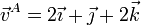
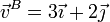
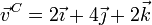
3 Caso I
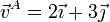
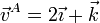
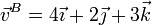
Tenemos las velocidades


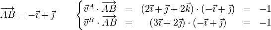
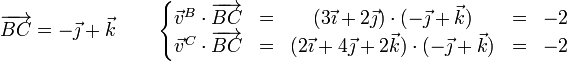
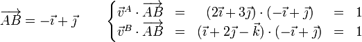
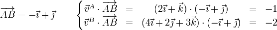
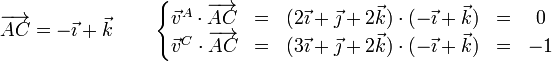
Comprobamos primero si se trata de un posible movimiento rígido, chequeando la condición de equiproyectividad para cada par de puntos
- Partículas A y B
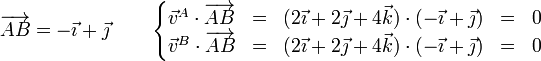
- Partículas A y C
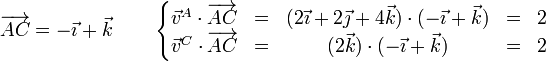
- Partículas B y C
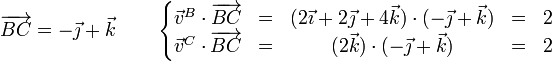
Se verifica en los tres casos, por lo que se trata de un movimiento posible para un sólido rígido.
A continuación, comprobamos si las tres velocidades son iguales. No lo son. Por tanto, no puede tratarse de una traslación o un estado de reposo.
Comprobamos ahora si hay dos velocidades iguales. Las hay. Esto quiere decir que el EIRMD es paralelo a la recta que pasa por los dos puntos con la misma velocidad. Para ver si se trata de una rotación, examinamos si cualquiera de las velocidades es perpendicular a esta dirección. No necesitamos volver a calcular nada, ya que lo hicimos previamente:
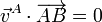
Por tanto se trata de un movimiento de rotación pura.
4 Caso II
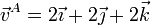
Tenemos las velocidades
Comprobamos la equiproyectividad
- Partículas A y B
- Partículas A y C
- Partículas B y C
De nuevo se verifica en los tres casos, por lo que se trata de un movimiento posible.
Puesto que las tres velocidades no son iguales, no puede tratarse de una traslación o un estado de reposo.
Comprobamos ahora si hay dos velocidades iguales. No las hay.
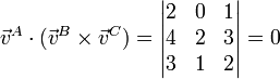
Verificamos entonces si las velocidades son coplanarias:
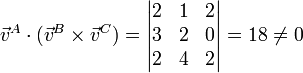
Por no se nulo, se trata de un movimiento helicoidal.
5 Caso III
El tercer caso

puede clasificarse por simple inspección. Puesto que las tres velocidades son iguales, y no nulas, se trata de un movimiento de traslación.
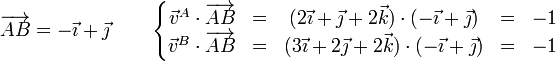
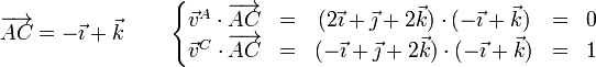
6 Caso IV
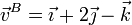
En este caso, las velocidades valen
Examinamos la condición de rigidez
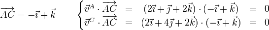
- Partículas A y B
- Partículas A y C

- Partículas B y C
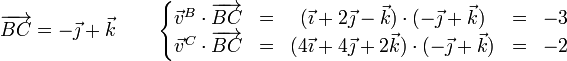
Puesto que no se cumple la condición de equiproyectividad, este caso es imposible como movimiento de un sólido rígido.
7 Caso V
En este caso, tenemos las velocidades
Examinamos la equiproyectividad
- Partículas A y B
- Partículas A y C
- Partículas B y C

De nuevo se verifica en los tres casos, por lo que se trata de un movimiento posible.
Las tres velocidades no son iguales, por lo que no puede tratarse de una traslación o un estado de reposo.
Comprobamos ahora si hay dos velocidades iguales. No las hay.
Verificamos entonces si las velocidades son coplanarias:
Puesto que se trata de vectores coplanarios, este movimiento es una rotación pura.
8 Caso VI
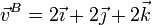
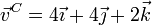
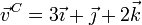
Por último, tenemos las velocidades,

Testeamos la condición de rigidez
- Partículas A y B
- Partículas A y C
No necesitamos continuar. Una vez que se viola la equiproyectividad podemos afirmar que se trata de un movimiento imposible para un sólido rígido.
9 Resumen
Reuniendo los resultados de los seis casos queda
| Caso | Estado |
|---|---|
| I | Rotación |
| II | Helicoidal |
| III | Traslación |
| IV | Imposible |
| V | Rotación |
| VI | Imposible |

