6.6. Disco en manivela ranurada

De Laplace

(Redirigido desde 7.6. Disco en manivela ranurada)

Contenido

1 Enunciado
2 Posición del CIR
3 Reducción cinemática
- 3.1 Directamente
- 3.2 Por composición de movimientos
  - 3.2.1 Velocidad
  - 3.2.2 Velocidad angular
4 Tipo de movimiento

1 Enunciado

El sistema de la figura está constituido por un plano vertical fijo $O X 1 Y 1$ (sólido “1”) que en todo instante contiene a otros dos sólidos en movimiento: un disco de radio $R$ y centro $C$ (sólido “2”), que rueda sin deslizar sobre el eje horizontal $O X 1$ ; y una manivela ranurada $O A$ (sólido “0”), que es obligada a girar con velocidad angular constante $Ω$ alrededor de un eje permanente de rotación que pasa por el punto $O$ y es perpendicular al plano fijo definido como sólido “1” (eje $O Z 1$ ). Los movimientos de ambos sólidos se hallan vinculados entre sí porque el centro C del disco está obligado a deslizar en todo instante a lo largo de la ranura de la manivela.

Considerando el movimiento {20} como el movimiento problema, se pide:

Haciendo uso de procedimientos gráficos, determinar la posición del CIR de dicho movimiento {20}.
Utilizando como parámetro geométrico el ángulo $θ$ indicado en la figura, obtener la reducción cinemática del movimiento {20} en el punto C, $\{\vec{\omega}_{20} (\theta), \vec{v}_{20}^{\, C} (\theta)\}$ .
Clasificar el movimiento {20} en el instante en que $θ = π / 2$ especificando si se trata de rotación, traslación, movimiento helicoidal o reposo.

2 Posición del CIR

Por el teorema de los tres centros, el CIR $I 20$ debe estar alineado con el $I 21$ y el $I 01$ .

Por tratarse de una rodadura sin deslizamiento, el CIR del movimiento {21} es el punto de contacto de la rueda con el eje horizontal.

El CIR del movimiento {01} es el punto O, de articulación de la manivela con el eje.

Por estar alineado con estos dos, el CIR del movimiento {20} debe encontrarse sobre el eje horizontal $O X 1$ . Queda por determinar dónde exactamente.

El vínculo de que el centro C del disco se encuentre sobre la manivela obliga a que la velocidad del punto C en el movimiento {20} sea necesariamente a lo largo de ésta. Puesto que el CIR se encuentra sobre la recta que pasa por C y es perpendicular a la velocidad $\vec{v}^C_{20}$ basta con trazar la perpendicular a la manivela en C. El punto donde esta recta corta al eje $O X 1$ es el CIR $I 20$ .

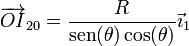
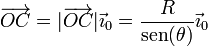
El vector de posición de este punto será de la forma

$\overrightarrow{OI}_{20}=x\vec{\imath}_1$

El valor de $x$ lo obtenemos aplicando trigonometría. El segmento $O I 20$ es la hipotenusa de un triángulo rectángulo cuyo cateto contiguo es $O C$ . Por tanto

$x = \left|\overrightarrow{OI}_{20}\right| = \frac{|\overrightarrow{OC}|}{\cos(\theta)}$

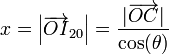
A su vez OC es la hipotenusa de un triángulo rectángulo cuyo cateto opuesto mide R, el radio del disco

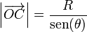
$\left|\overrightarrow{OC}\right| = \frac{R}{\mathrm{sen}(\theta)}$

Por tanto

$\overrightarrow{OI}_{20}=\frac{R}{\mathrm{sen}(\theta)\cos(\theta)}\vec{\imath}_1$

3 Reducción cinemática

3.1 Directamente

3.1.1 Velocidad

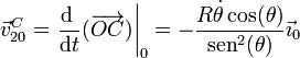
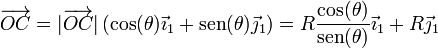
La velocidad de C la podemos hallar derivando el vector de posición en un sistema de referencia “0” ligado a la manivela. Tomando como eje $O X 0$ el que va a lo largo de la manivela, el vector de posición relativo es

$\overrightarrow{OC}=|\overrightarrow{OC}|\vec{\imath}_0 = \frac{R}{\mathrm{sen}(\theta)}\vec{\imath}_0$

Derivando en esta expresión

$\vec{v}^C_{20}=\left.\frac{\mathrm{d}\ }{\mathrm{d}t}(\overrightarrow{OC})\right|_0 = -\frac{R\dot{\theta}\cos(\theta)}{\mathrm{sen}^2(\theta)}\vec{\imath}_0$

3.1.2 Velocidad angular

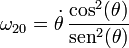
Puesto que conocemos la posición del CIR $I 20$ podemos hallar la velocidad angular empleando la relación

$\vec{v}^C_{20}=\omega_{20}\vec{k}\times\overrightarrow{I_{20}C}$

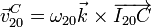
El vector de posición relativo desde el CIR va en la dirección del eje $O Y 0$ y tiene por módulo el cateto opuesto de un triángulo rectángulo

$\overrightarrow{I_{20}C}=|\overrightarrow{OI_{20}}|\mathrm{sen}(\theta)\vec{\jmath}_0 = \frac{R}{\cos(\theta)}\vec{\jmath}_0$

Por tanto,

$-\frac{R\dot{\theta}\cos(\theta)}{\mathrm{sen}^2(\theta)}\vec{\imath}_0 = \omega_{20}\vec{k}\times\left(\frac{R}{\cos(\theta)}\vec{\jmath}_0\right)=-\frac{\omega_{20}R}{\cos(\theta)}\vec{\imath}_0$

Despejando

$\omega_{20}=\dot{\theta}\,\frac{\cos^2(\theta)}{\mathrm{sen}^2(\theta)}$

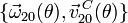
3.1.3 Expresión de la reducción cinemática

Reuniendo los dos resultados obtenemos la reducción cinemática

$\left\{\vec{\omega}_{20},\vec{v}^C_{20}\right\}=\left\{\dot{\theta}\,\frac{\cos^2(\theta)}{\mathrm{sen}^2(\theta)}\vec{k},-\frac{R\dot{\theta}\cos(\theta)}{\mathrm{sen}^2(\theta)}\vec{\imath}_0\right\}$

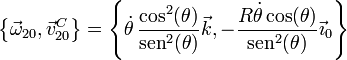
Empleando la base ligada al sólido “1”, esto queda

$\left\{\vec{\omega}_{20},\vec{v}^C_{20}\right\}=\left\{\dot{\theta}\,\frac{\cos^2(\theta)}{\mathrm{sen}^2(\theta)}\vec{k},-\frac{R\dot{\theta}\cos(\theta)}{\mathrm{sen}^2(\theta)}(\cos(\theta)\vec{\imath}_1+\mathrm{sen}(\theta)\vec{\jmath}_1)\right\}=\left\{\dot{\theta}\,\frac{\cos^2(\theta)}{\mathrm{sen}^2(\theta)}\vec{k},-\frac{R\dot{\theta}\cos^2(\theta)}{\mathrm{sen}^2(\theta)}\vec{\imath}_1-\frac{R\dot{\theta}\cos(\theta)}{\mathrm{sen}(\theta)}\vec{\jmath}_1\right\}$

3.2 Por composición de movimientos

3.2.1 Velocidad

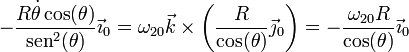
Alternativamente, podemos obtener la velocidad de C empleando la fórmula de composición de velocidades

$\vec{v}^C_{20}=\vec{v}^C_{21}+\vec{v}^C_{10}=\vec{v}^C_{21}-\vec{v}^C_{01}$

La velocidad en el movimiento {01} corresponde a una rotación alrededor de O

$\vec{v}^C_{01}=\omega_{01}\vec{k}\times\overrightarrow{OC}$

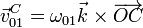
siendo su velocidad angular

$\omega_{01}=\dot{\theta}$

y el vector de posición

$\overrightarrow{OC}=|\overrightarrow{OC}|\left(\cos(\theta)\vec{\imath}_1+\mathrm{sen}(\theta)\vec{\jmath}_1\right) = R\frac{\cos(\theta)}{\mathrm{sen}(\theta)}\vec{\imath}_1+R\vec{\jmath}_1$

lo que nos da la velocidad

$\vec{v}^C_{01}=R\dot{\theta}\left(-\vec{\imath}_1+\frac{\cos(\theta)}{\mathrm{sen}(\theta)}\vec{\jmath}_1\right)$

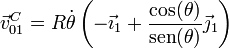
La velocidad de C en el movimiento {21} la podemos hallar derivando la posición en el sistema “1”, que conocemos en todo momento

$\vec{v}^C_{21}=\left.\frac{\mathrm{d}\ }{\mathrm{d}t}(\overrightarrow{OC})\right|_1 = -\frac{R\dot{\theta}}{\mathrm{sen}^2(\theta)}\vec{\imath}_1$

Resulta una velocidad horizontal como corresponde a que el punto C se desplaza paralelamente al eje $O X 1$ .

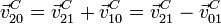
Componiendo las dos velocidades

$\vec{v}^C_{20}= -\frac{R\dot{\theta}}{\mathrm{sen}^2(\theta)}\vec{\imath}_1 - R\dot{\theta}\left(-\vec{\imath}_1+\frac{\cos(\theta)}{\mathrm{sen}(\theta)}\vec{\jmath}_1\right) = -R\dot{\theta}\,\frac{\cos^2(\theta)}{\mathrm{sen}^2(\theta)}\vec{\imath}_1-R\dot{\theta}\frac{\cos(\theta)}{\mathrm{sen}(\theta)}\vec{\jmath}_1$

3.2.2 Velocidad angular

Igualmente, podemos hallar la velocidad angular del movimiento {20} como

$\omega_{20}=\omega_{21}-\omega_{01}\,$

siendo

$\omega_{01}=\dot{\theta}$

La velocidad angular del movimiento {21} la podemos hallar a partir de la velocidad de C

$\vec{v}^C_{21}=\omega_{21}\vec{k}\times\overrightarrow{I_{21}C}=\omega_{21}\vec{k}\times(R\vec{\jmath}_1)=-R\omega_{21}\vec{\imath}_1$

Igualando esta expresión a la velocidad lineal calculada anteriormente y despejando queda

$\omega_{21}=\frac{\dot{\theta}}{\mathrm{sen}^2(\theta)}$

Llevando esto a la fórmula de composición de velocidades angulares, llegamos a

$\omega_{20}=\frac{\dot{\theta}}{\mathrm{sen}^2(\theta)}-\dot{\theta}=\frac{\dot{\theta}\cos^2(\theta)}{\mathrm{sen}^2(\theta)}$

Reuniendo la velocidad y la velocidad angular nos queda la misma reducción cinemática que ya expresamos anteriormente.

4 Tipo de movimiento

Cuando $θ = π / 2$ , la reducción cinemática se reduce a

$\left\{\vec{\omega}_{20},\vec{v}^C_{20}\right\}=\left.\left\{\dot{\theta}\,\frac{\cos^2(\theta)}{\mathrm{sen}^2(\theta)}\vec{k},-\frac{R\dot{\theta}\cos(\theta)}{\mathrm{sen}^2(\theta)}(\cos(\theta)\vec{\imath}_1+\mathrm{sen}(\theta)\vec{\jmath}_1)\right\}\right|_{\theta=\pi/2}=\{\vec{0},\vec{0}\}$

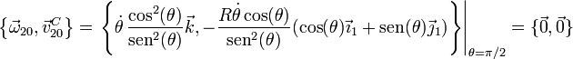
y por tanto el disco se encuentra instantáneamente en reposo respecto a la manivela.

6.6. Disco en manivela ranurada

De Laplace

Contenido

1 Enunciado

2 Posición del CIR

3 Reducción cinemática

3.1 Directamente

3.1.1 Velocidad

3.1.2 Velocidad angular

3.1.3 Expresión de la reducción cinemática

3.2 Por composición de movimientos

3.2.1 Velocidad

3.2.2 Velocidad angular

4 Tipo de movimiento

Herramientas:

Buscar

Vistas

Herramientas

Herramientas personales

Navegación

SEARCH

TOOLBOX

LANGUAGES